Forecasting House Price Growth Using Months Supply of Housing
Key Takeaways
- This article proposes forecasting house price growth using months supply of housing.
- Some of the theoretical reasons one might expect months supply to be relevant for house price growth include referential and momentum-based pricing, a relative lack of new construction in the short run, and its inherent inclusion of variables that affect the home-buying market, such as interest rates and unemployment.
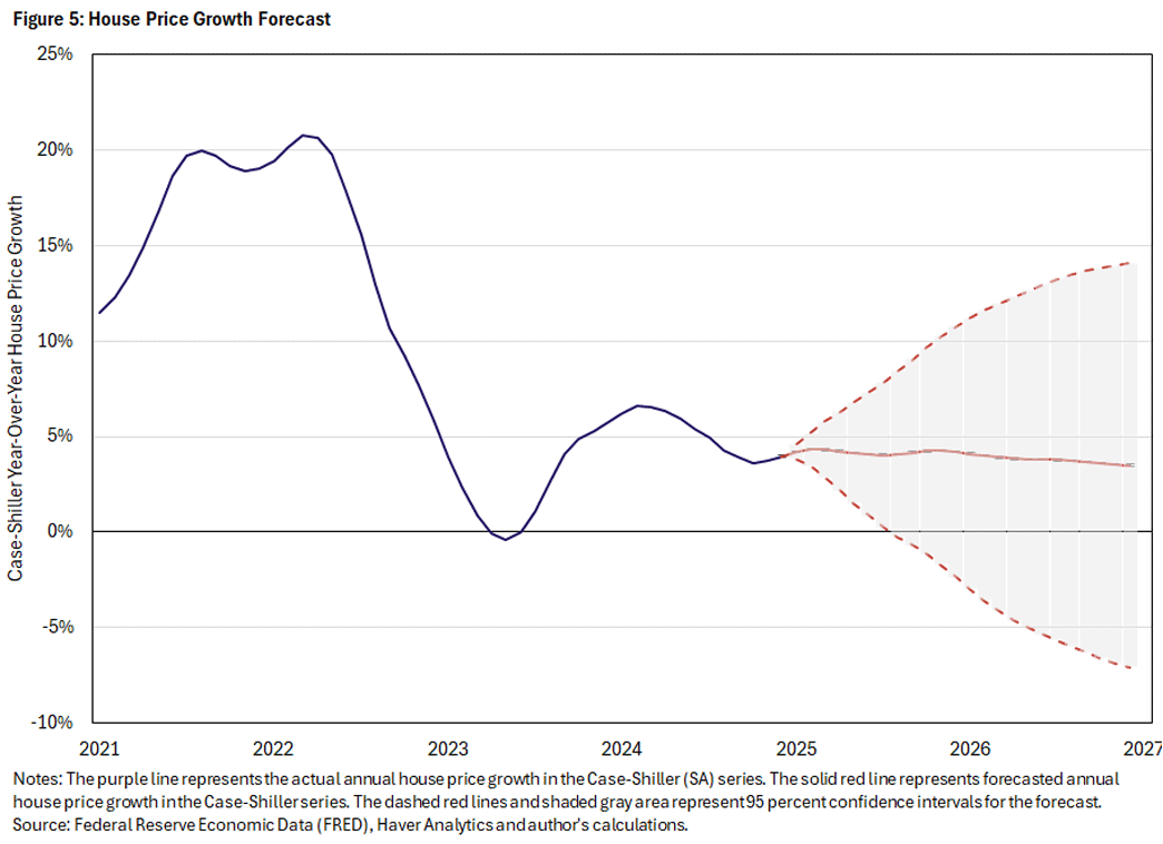
- House price growth is projected to be stable over the next year, although substantial uncertainty persists.
House prices are of keen interest to policymakers, economists, industry professionals and homebuyers. Naturally, forecasting the direction of house prices receives considerable attention. In this article, we'll examine a specific metric that has a robust ability to predict house price growth: months supply.
Months supply is the number of houses available for sale divided by the number of houses sold per month. For example, if months supply is 6, it would take six months to sell all of the current inventory, assuming no additional houses were added and the sales per month did not change. Since the sales rate is the number of houses sold per month divided by the number of houses available for sale, months supply is also the inverse of the sales rate.
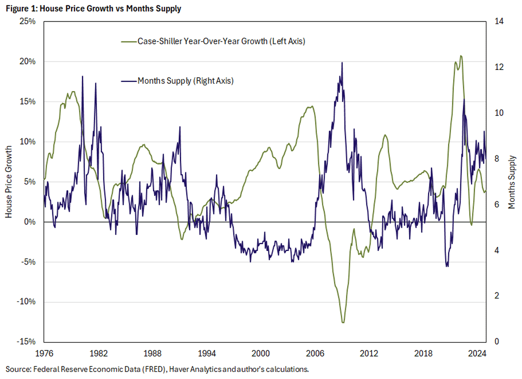
Figure 1 compares months supply of new homes to house price growth.1 One can see that house price growth tends to slow when months supply shoots up. Conversely, house price growth tends to accelerate when months supply falls. This correlation suggests a role for months supply in forecasting house price growth.
Theoretical Considerations
There are sound theoretical reasons to expect months supply to help forecast house price growth.
Referential and Momentum-Based Pricing
No two houses are the same, and so determining the fair value of a house involves guess work. Sellers assess their homes against comparable, recently sold ones to try to determine what their houses might fetch. This leads to referential pricing and momentum-based pricing.2
This experimentation in price-setting has implications for both sellers and buyers regarding the importance of months supply. Sellers may set overly high prices and only discover they're too high when houses sell slowly, which in turn leads to lower prices at an individual level. Thus, longer time on the market in the aggregate — or larger months supply — leads to lower prices at an aggregate level.
Conversely, sellers can set overly low prices (if demand has suddenly increased, for instance), which leads to houses selling quickly and for more than the prices originally asked. As those above-asking-price transactions roll in, other sellers ask for high prices. So fast sales rates — or smaller months supply — lead to high house price growth.
New Construction
The idea of using months supply to gauge house price growth is reinforced by construction's inability to meaningfully alter the supply of housing in the short run. It takes months to build houses, and developers cannot adjust to changes in demand rapidly. Additionally, the flow of houses developers can bring to market is only a small percentage of the usual sales volume, as the vast majority comes from existing homeowners. So, the experimentation by homeowners discussed above in large part determines properties of the whole market.
Outside Influences
Factors affecting demand or supply — such as interest rates, rent inflation, expected house price growth and unemployment — should show up in buying and selling dynamics, making months supply akin to a sufficient statistic for house price growth.
Empirical Evidence on Using Months Supply
These theoretical considerations suggest that house price growth and months supply should be inversely correlated and that months supply should lead house price growth. Empirical evidence supports both predictions.
Regarding the first prediction, Figure 1 confirms that house price growth and months supply are inversely correlated. The correlation is not extreme at -0.38, but the relationship is obvious. In the 2000s, when months supply was exceptionally tight (four months), house prices grew in a high and sustained manner. In the housing crisis of 2007-09, months supply exploded, while house price growth came crashing down. And this is not a modern phenomenon either, as the 1970s and 1980s display the same patterns.
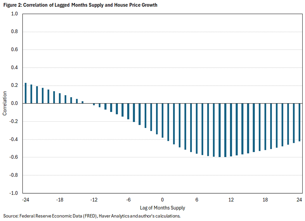
Examining the second prediction — that months supply should lead house price growth — there are several clear instances where this is true. For instance, in June 2020, the exceptionally tight months supply preceded the largest house price growth on record. However, this claim can be supported more systematically. Figure 2 shows the correlation between a certain lag of months supply and Case-Shiller house price growth. The correlation with a lag of 10 months is the largest in absolute value, reaching -0.60. This suggests a strong lead-lag relationship with months supply predicting house price growth, as it implies that months supply at a 10-month lag explains 36 percent (denoted by an R2 of 0.36, or (-0.6)2) of the variation in house price growth.
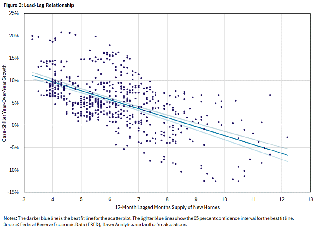
The 12-month-lag correlation is only slightly smaller, so Figure 3 shows the lead-lag relationship in a scatter plot of the 12-month lagged supply of new homes against the 12-month Case-Shiller house price growth rate, along with a best fit line and confidence interval. The negative relationship is clearly apparent. But there are also many deviations from the best fit line, reflecting that all sorts of shocks (including shocks that feed into months supply) can happen over the next year, which fundamentally limits how well house price growth can be predicted.
Why Months Supply and Not Other Variables?
At this point, focusing on months supply might seem arbitrary. However, months supply does better at predicting house price growth than many other relevant variables, such as the unemployment rate, the price-rent ratio, the 10-year Treasury yield, inflation, time trends and the share of the population with an age of 25-54 (commonly known as the prime-age population).
One way to see this is to regress these variables on next year's Case-Shiller house price growth, as seen in Table 1. Projecting just months supply explains 34.7 percent of house price growth (slightly less than the 36 percent at the optimal lag length). Adding the current Case-Shiller growth rate significantly increases explanatory power to 59.2 percent. Demographics (the prime-age population share) also contribute a bit, increasing the explanatory power from 59.2 percent to 69.6 percent. After that, additional variables (while sometimes statistically significant) add little.3
| (1) | (2) | (3) | (4) | (5) | (6) | (7) | (8) | |
|---|---|---|---|---|---|---|---|---|
| Months supply (new) | -2.00* | -1.38* | -1.92* | -1.73* | -1.51* | -1.46* | -1.37* | -1.38* |
| Case-Shiller (y/y %) | 0.52* | 0.34* | 0.41* | 0.46* | 0.51* | 0.53* | 0.51* | |
| Pop. share age 25-54 | -101.2* | -90.6* | -83.6* | -73.7* | -76.6* | -81.7* | ||
| Price-rent ratio (2000=100) | -0.064* | -0.091* | -0.082* | -0.082* | -0.066* | |||
| Ten-year treasury yield (%) | -0.18* | -0.22* | -0.17* | -0.29* | ||||
| Unemployment (%) | 0.33* | 0.32* | 0.28* | |||||
| CPI inflation (y/y %) | -12 | -15.1 | ||||||
| Time (months) | -0.0041 | |||||||
| Observations | 588 | 576 | 576 | 576 | 576 | 576 | 576 | 576 |
| R-squared | 0.347 | 0.592 | 0.696 | 0.723 | 0.728 | 0.734 | 0.735 | 0.736 |
| Note: The dependent variable in each specification is the Case-Shiller annual house price growth (SA). A constant is included in each specification, but its value is not reported. * p<.0001 Source: Author's calculations. |
||||||||
The importance of months supply is robust. In the preceding exercise, the order in which variables are added to the regressions above affects the incremental increase in explanatory power (or R2) that each variable gives. An alternative way is to specify many regression models (one for each possible ordering) and compute the incremental R2 relative to the maximum possible R2 (which arises from including all the variables).4 The results of this decomposition are given in Table 2 and show that the two most important explanatory variables are the current Case-Shiller growth rate (achieving 39.2 percent of the maximum) and months supply (achieving 32.9 percent of the maximum). The other variables are far less important, although demographics matter somewhat.5 These results suggest the focus on months supply is quite reasonable.
| Variable | Contribution |
|---|---|
| Unemployment (%) | 1.6 |
| 10-year treasury yield (%) | 2.5 |
| Pop. share age 25-54 | 13.5 |
| Months supply (new) | 32.9 |
| Case-Shiller (y/y %) | 39.2 |
| Price-rent ratio (2000=100) | 4.4 |
| CPI inflation (y/y %) | 3.1 |
| Time (months) | 2.8 |
| Source: Author's calculations. | |
Forecasting House Price Growth
Turning to forecasting, I choose a VAR specification of annual Case-Shiller house price growth and months supply of new houses.6 While additional variables could be added, these are less important, and this simple specification highlights the predictive power of months supply.
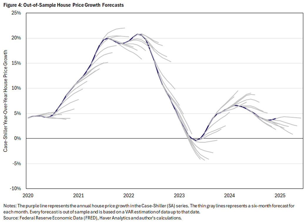
To assess model performance, I construct an out-of-sample forecast at each point of time using only data up to that time, starting with 2020. The results of this exercise are shown in Figure 4. This is obviously an exceptionally hard period to forecast, as many shocks — unemployment, supply chain, fiscal and monetary — hit the economy throughout this period. However, the forecasts detect the turning points and trends well, despite being parsimonious. In this respect, the forecasting model is a substantial success.
Since the model's out-of-sample forecasting ability is substantial, it is worthwhile to consider the forecast for the short-to-medium term, shown in Figure 5. The forecast essentially says the housing market (based on the most recent data from December 2024) is in a stable place with expected house prices projected to be flat. Given that house price growth rates have been bouncing around 5 percent the last few years, and months supply is somewhat elevated but not very high, this seems like a reasonable prediction.
As with all forecasting models, as time goes on, the cumulative effect of shocks hitting the economy leads to reduced confidence. At the end of the year, statistically there's a 5 percent chance that annual housing inflation will be greater than 12 percent or less than -3 percent. Given the drastic fluctuations we've seen in house prices in the past, this lack of confidence in longer-term projections seems prudent.
Grey Gordon is a senior economist in the Research Department at the Federal Reserve Bank of Richmond.
There are two main measures of months supply, one for new homes and one for existing homes. Months supply of existing homes has a trend and shorter sample than new homes. It also has worse predictive power for house price growth. So for this article I focus on months supply of new homes.
See the 2019 paper "Home Price Expectations and Behaviour: Evidence From a Randomized Information Experiment" by Luis Armona, Andreas Fuster and Basit Zafar.
I use a very high bar for statistical significance in this table (a p-value of .0001) to show the robustness of relationships without reporting t-statistics or standard errors.
This procedure is known as the Shapley-Owen decomposition.
The share of 25-54-year-olds undulates at low frequency, so its predictive power is difficult to interpret. It may have just been lucky in peaking during the late 1990s and beginning a relatively rapid descent around 2010. This feature — with the small explanatory power relative to months supply — leads me to omit it from the forecasting model. Parsimony in the forecasting model is necessary to prevent the number of coefficients from exploding.
I choose a lag length of 11, which maximizes the AIC criterion.
To cite this Economic Brief, please use the following format: Gordon, Grey. (March 2025) "Forecasting House Price Growth Using Months Supply of Housing." Federal Reserve Bank of Richmond Economic Brief, No. 25-11.
This article may be photocopied or reprinted in its entirety. Please credit the author, source, and the Federal Reserve Bank of Richmond and include the italicized statement below.
Views expressed in this article are those of the author and not necessarily those of the Federal Reserve Bank of Richmond or the Federal Reserve System.
Receive a notification when Economic Brief is posted online.


